Early Prediction for Fatty Liver Disease with Eigenvector-Based Feature Selections for Model Performance Enhancement
2 Department of Family medicine, College of Medicine, National Taiwan University, Taipei, Taiwan, Email: bretthuang@ntu.edu.tw
3 Department of Computer Science and information Engineering, National Taiwan University, Taipei, Taiwan, Email: flai@ntu.edu.tw
Received: 05-Aug-2021 Accepted Date: Aug 22, 2021 ; Published: 31-Aug-2021
Citation: Liu JH, Huang KC, Lai F (2021). Early Prediction Model for Fatty Liver Disease with Eigenvector-Based Feature Selections for Input Optimization and LSTM Related Classifiers for Performance Enhancement. EJBI. 17(8): 18-34.
This open-access article is distributed under the terms of the Creative Commons Attribution Non-Commercial License (CC BY-NC) (http://creativecommons.org/licenses/by-nc/4.0/), which permits reuse, distribution and reproduction of the article, provided that the original work is properly cited and the reuse is restricted to noncommercial purposes. For commercial reuse, contact submissions@ejbi.org
Abstract
Objectives: This study is aimed to achieve the rapid optimization of the input feature subset that satisfies the expert’s point of view and enhance the prediction performance of the early prediction model for fatty liver disease (FLD).
Methods: We explore a large-scale and high-dimension dataset coming from a northern Taipei Health Screening Center in Taiwan, and the dataset includes data of 12,707 male and 10,601 female patients processed from around 500,000 records from year 2009 to 2016. We propose three eigenvector-based feature selections taking the Intersection of Union (IoU) and the Coverage to determine the sub-optimal subset of features with the highest IoU and the Coverage automatically, use various long short-term memory (LSTM) related classifiers for FLD prediction, and evaluate the model performance by the test accuracy and the Area Under the Receiver Operating Characteristic Curve (AUROC).
Results: Our eigenvector-based feature selection EFSTW has the highest IOU and the Coverage and the shortest total computing time. For comparison, the highest IOU, the Coverage, and computing time are 30.56%, 45.83% and 260 seconds for female, and that of a benchmark, sequential forward selection (SFS), are 9.09%, 16.67% and 380,350 seconds. The AUROC with LSTM, biLSTM, Gated Recurrent Unit (GRU), Stack-LSTM, Stack-biLSTM are 0.85, 0.86, 0.86, 0.86 and 0.87 for male, and all 0.9 for female, respectively.
Conclusion: Our method explores a large-scale and high-dimension FLD dataset, implements three efficient and automatic eigenvector-based feature selections, and develops the model for early prediction of FLD efficiently.
https://maviyolculuk.online/
https://mavitur.online/
https://marmaristeknekirala.com.tr
https://tekneturumarmaris.com.tr
https://bodrumteknekirala.com.tr
https://gocekteknekirala.com.tr
https://fethiyeteknekirala.com.tr
Keywords
Fatty liver disease; Eigenvector; Feature selection; Intersection over union; Long short-term memory
Introduction
Types of FLD, Dataset Retrieval Status and Literature Review of FLD Prediction
Prior research on machine learning for early disease prediction has focused on diabetes, FLD, hypotension, and other metabolic syndromes [1]. Although FLD has no notable symptoms, it may progress to severe liver diseases. If not treated within three years, the possibility for FLD to develop into nonalcoholic steatohepatitis (NASH) and liver cirrhosis is 25% and 10-25% [1,2]. Moreover, FLD increases the prevalence of diabetes, metabolic syndrome, and obesity, creating enormous medical and economic burdens for society. It raises the urgent need for early and precise prediction of FLD, followed by personalized treatment and recommendations.
Typically, FLD is classified into two types according to its cause: alcohol-related fatty liver disease (AFLD) and nonalcoholic fatty liver disease (NAFLD). AFLD is commonly caused by excessive alcohol consumption, whereas NAFLD is due to other more complex factors. Although most prior research has focused on NAFLD prediction rather than AFLD [3-7], there is no inherent reason to conduct separate prediction processes. The preceding research focus on NAFLD is partly due to the datasets being insufficiently large to predict both types of FLD.
Besides, as shown in Table 1, dataset used in this study is much larger and covers a much larger period, and previous studies [7-10] have relied on techniques such as leave-one-out (LOO) cross validation to accommodate these small datasets with sample sizes and short periods to avoid overfitting [3-9]. They conducted feature selection through human intervention [10-14] rather than by automation that is not a common practice in machine learning. The use of such limited datasets raises the likelihood that the identified models are at risk of overfitting, and their short duration makes it difficult to perform the prediction possible in this study using an eight-year dataset.
| Item for Comparison | Sample Size | Date Time Duration | Feature Selection | FLD Types | Gender Types | Prediction of Future Health | Source of Dataset |
|---|---|---|---|---|---|---|---|
| Authors and Title | |||||||
| Birjandi et al., ‘Prediction and Diagnosis of Non-Alcoholic Fatty Liver Disease (NAFLD) and Identification of Its Associated Factors Using the Classification Tree Method’, 2016 | 1,700 | 2012 | Yes | NAFLD | Male/ Female | No | Health Houses |
| Raika et al., ‘Prediction of Non-alcoholic Fatty Liver Disease Via a Novel Panel of Serum Adipokines’, 2016 | <100 | 2012∼2014 | No | NAFLD | Male | No | Hospital |
| Yip et al., ’Laboratory parameter-based machine learning model for excluding non-alcoholic fatty liver disease (NAFLD) in the general population’, 2017 | <1,000 | 2015 | Yes | NAFLD | Male | No | Hospital |
| Islam et al., ‘Applications of Machine Learning in Fatty Live Disease Prediction’, 2018 | <1,000 | 2012∼2013 | Yes | NAFLD/ AFLD | Male/ Female | No | Hospital |
| Ma et al., ‘Application of Machine Learning Techniques for Clinical Predictive Modelling: A Cross-Sectional Study on Non-alcoholic Fatty Liver Disease in China’, 2018 | <11,000 | 2010 | Yes | NAFLD | Male/ Female | No | Hospital |
| Wu et al., ‘Prediction of fatty liver disease using machine learning algorithms’, 2019 | <600 | 2009 | No | NAFLD/ AFLD | Male | No | Hospital |
| Present Task | >150,000 | 2009∼2016 | Yes | NAFLD/ AFLD | Male/ Female | Yes | Health Screening Center |
Table 1: Comparison of prior research and present study for FLD prediction.
Recently, machine learning models have been used extensively in medicine and healthcare for fixed-length input data. In contrast, long short-term memory (LSTM) -related models can process the variable-length data of large-scale and high-dimension dataset resulted from different patient‘s irregular examining periods for future prediction, although time-consuming. Accordingly, the contribution of this paper is that we explore a large-scale dataset with high dimensionality for FLD prediction, propose and implement the efficient feature selections to select features close to expert-selected ones automatically and rapidly, and develop the prediction models using various LSTM-related classifiers with fixed-interval timestamps for FLD prediction.
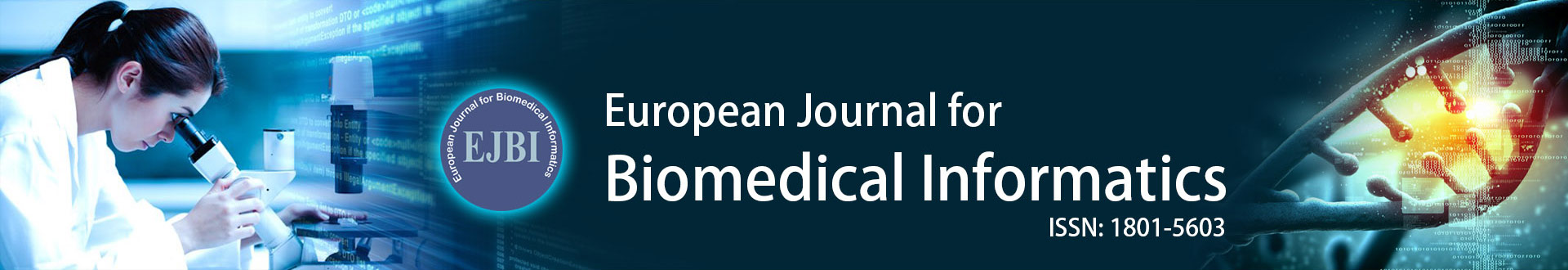
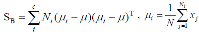
Techniques for Dimensionality ReductionConcept of principal component analysis: Principal Component Analysis (PCA) is based on K-L transformation, and it can be used to visualize the structure of the original data on a lower dimensional space (in general, 2 or 3). The basic approach is to compute the eigenvectors of the covariance matrix computed from the original data corresponding to the few largest eigenvalues, and the processes are shown in formulas 1 to 4. The training dataset A = (a1,a2,...,ai,...,aN) = represents a n× N data matrix, where each ai is a normalized feature vector of dimension n for a sample, and N is the number of samples. PCA can be considered as a linear transformation from the original vectors of dataset to a projection feature vector as
 (1)
(1)
 (2)
(2)
 (3)
(3)
Where Y is a m * N feature vector matrix, m is the dimension of the feature vector, and transformation matrix W is a n * m transformation matrix whose columns are the eigenvectors corresponding to the m largest eigenvalues of the total scatter matrix S. Also, the mean dataset of all samples is shown in formula 3.
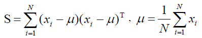
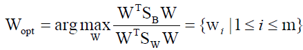
After applying the linear transformation WT, the scatter of the transformed feature vector {y1, y2,..., yN} is WTSW. In the PCA, the projection Wopt is chosen to maximize the determinant of the total scatter matrix of the projected samples as
 (4)
(4)
Where wi is the set of n-dimensional eigenvectors of S corresponding to m << n largest eigenvalues. That means, the input vector in an n-dimensional space is reduced to a feature vector in an m-dimensional subspace.
Concept of linear discriminant analysis
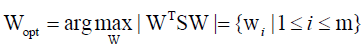
Linear discriminant analysis (LDA) uses class specific information which best discriminates among classes. LDA produces an optimal linear discriminant function which maps the input data into the classification space, the class identification of this sample is decided based on some metrics such as Euclidean distance, and it selects W such that the ratio of the between-class scatter matrix SB and the within-class scatter Sw of the training dataset is maximized. The processes are shown in formulas 5 to 9.
Assuming that Sw is non-singular, the basis vectors in W correspond to the first m eigenvectors with the largest eigenvalues of S-1W− SB.
 (5)
(5)
 (6)
(6)
 (7)
(7)
Where Ni is the number of training samples in class i, c is the number of distinct classes, and μi μ is the mean vector of samples belonging to class i. The optimal projection Wopt is chosen as follows.
 (8)
(8)
Where wi is the set of generalized eigenvectors of SB and SW corresponding to the largest generalized engienvalues of λi, such that
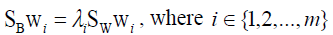 (9)
(9)
Applications using the combination of PCA and LDA: The combination of PCA and LDA has reached to be state-of-theart in the image recognition field, especially the prediction of face, gender, face expression recognition, electromyography (EMG) recognition in bionic mechanical control, and banknote discrimination [15-22]. The superior performance of this combination of PCA and LDA in previous studies leads us to use it for feature reduction to our numerical, heterogeneous largescale and high-dimension dataset of FLD that consists of lab tests and questionnaires.
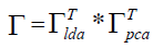
The projecting matrix Γ is the combination of PCA and LDA space that can be calculated by formula 10 listed below.
 (10)
(10)
Where in 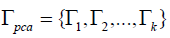 is the projecting matrix of the PCA
space, and
is the projecting matrix of the PCA
space, and 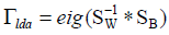 (in applications, SW is in general
degenerate and its inverse does not exist) is the eigenvector
corresponding to the eigenvalues, and wherein SW is the inverse
matrix of within-class scatter matrix and SB is the between-class
scatter matrix.
(in applications, SW is in general
degenerate and its inverse does not exist) is the eigenvector
corresponding to the eigenvalues, and wherein SW is the inverse
matrix of within-class scatter matrix and SB is the between-class
scatter matrix.
Feature selection is an essential step in machine learning that identify a feature subset to construct a better model requiring less computing time for training and testing. Frequently used feature selections involve the wrapper-based, the filter-based, and the embedded methods. Wrapper-based methods use a classifier to score the feature subsets, i.e., it selects features based on classification accuracy, but time-consuming. Filter-based methods use a proxy measure instead of accuracy to score a feature subset, which is efficient but does not always produce a good model since it seldom relates to classification accuracy [23]. Embedded methods perform feature selection as part of the model construction process, which tends to be one of two types of mentioned methods in accuracy and computational complexity [24-26].
Conventional but accurate wrapper-based method, SFS [27], aka Whitney’s method in Pattern Recognition (PR), can test the relevance of signals or measure by considering the relationships between them. It starts with an empty set and selects the first best feature among m features, i.e., the one with the highest recognition rate, available at that moment. Then, it selects one among m-1 features to combine the first feature with the jointly highest recognition rate. Liu et al. [28] conclude that SFS is time-consuming and inefficient when processing a large-scale and high-dimension dataset.
Features Suggested by Experts for FLD PredictionThere are many risk factors related to FLD but not all of preceding research adopts the feature selection automatically. For example, Wu et al. [7] manually selected only ten features from the collected data in a manner of human intervention. In contrast, in this study the experts have suggested at least 24 features included in lab tests and questionnaires as a comparison basis for preventing the human intervention. Herein we only show some essential features in lab test in Table 2, and those included in questionnaire, such as ‚The ratio of GOT/GPT‘, ‚How many servings of bread do you eat?‘, ‚The metabolic equivalent for exercise per week‘, and ‚Have you smoke or not?‘, are not shown for brevity.
| Statistics | Males (n=88,056) (NFLD, FLD) = (34,885, 53,171) |
Females (n=72,564) (NFLD, FLD) = (48,574, 23,990) |
||
|---|---|---|---|---|
| Features | Mean | Std. | Mean | Std. |
| Age | 44.15 | 12.39 | 45.08 | 12.87 |
| BMI (Body Mass Index) |
24.63 | 3.38 | 22.39 | 3.49 |
| CH | 3.89 | 0.93 | 3.11 | 0.80 |
| CHOL (mg/dl) | 196.69 | 34.58 | 194.55 | 34.63 |
| Drink Alc. gram (Alcohol per Gram) |
12.82 | 43.48 | 1.94 | 16.13 |
| FAT (Body Fat) | 24.13 | 5.50 | 29.71 | 6.80 |
| FG (mg/dl) | 104.65 | 20.55 | 99.31 | 18.33 |
| GGR | 0.87 | 0.31 | 1.15 | 0.35 |
| GPT (IU/L) | 35.39 | 30.23 | 21.75 | 20.03 |
| HDLC (mg/dl) | 52.44 | 11.65 | 65.15 | 15.05 |
| LDLC (mg/dl) | 120.34 | 31.03 | 111.09 | 30.74 |
| Metaequi | 14.58 | 22.80 | 12.84 | 19.26 |
| TG (mg/dl) | 136.60 | 108.90 | 93.84 | 65.84 |
| WC (cm) | 83.81 | 8.77 | 72.19 | 8.13 |
| WHR | 0.87 | 0.06 | 0.77 | 0.06 |
| WEI (kg) | 71.83 | 11.33 | 55.81 | 8.97 |
Table 2: Important features and number of samples in FLD dataset
Applications of LSTM-Related ClassifiersConventional Recurrent Neural Networking (RNN) is the first architecture proposed to handle the concept of timestamp, but it can only remember the information from the previous time. LSTM is a kind of RNNs but it can learn long-term dependencies or more extended period historical information because of a memory function. Recent studies [29-34] show various applications in prediction using LSTM-based framework or model, and the superior performance of LSTM in them leads us to use it for our FLD prediction.
Method
Flowchart of FLD Prediction
This paper explores the steps of data preprocessing and cleaning, performing feature selection, and performing the prediction of FLD using LSTM related classifiers. We show the entire workflow for FLD prediction and those steps in Figures 1 to 3, and describe the content in detail in the remains of this chapter.

Figure 1: Flowchart of proposed FLD prediction.
Figure 2: Interpolation for the questionnaire features between any two medical checkups.
Figure 3: Flowcharts of FLD prediction with proposed eigenvector-based feature selections for different classifiers.
Data Preprocessing and Cleaning
We conduct the data preprocessing and cleaning procedure including the steps of handling missing value, performing interpolation, feature options simplification, feature conversion, and useless feature deletion, and handling gender dependency features.
To prepare the features set for LSTM, we perform interpolation to create monthly features between any two health exams for each subject. For numeric lab test features, we use spline interpolation with‚ piecewise cubic‘, and for questionnaire features with categorical values of integers, we use linear interpolation and then perform round-off to the nearest labels as shown in Figure 2. In feature options simplification, some multiple options for questionnaire features will be changed to binary options before model training since our model is the binary prediction.
To simplify the questionnaires‘ complexity, we convert the ‚grams of alcohol‘ comes from different questionnaires like ‚kind of drink‘, ‚habit of drink‘, ‚drink or not‘, and ‚alcohol density‘. Similarly, the ‚weekly exercise metabolic equivalent‘ comes from questionnaires of ‚kind of sport‘, ‚frequency of sport‘, and ‚time for sport‘. Besides, to the useless feature, we drop the features that are unrelated to FLD but other diseases such as ‚Cervical cancer‘, ‚Chinese medicine‘, and so on.
Automatic eigenvector-based Feature Selections
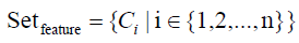
To evaluate the similarity or degree of consistency between the features selected from our methods and those suggested by experts and to strike a balance between efficiency and effectiveness, it performs the feature selections and compares the result by the measures, intersection of union (IOU) and the Coverage in this study. As shown in Figures 3, to 5, we use different eigenvectorbased feature selections in a technique such as bagging or voting that has parallel style and different classifiers, and it determines the sub-optimal subset of features with the highest value of IoU and Coverage automatically and unionizes the groups of features with the same value of Coverage when they have same value of IoU.
Figure 4: Steps of performing PCA and then LDA.
Figure 5: Step of determining the contribution or importance of features.
The formula and definition of IoU and Coverage are listed as follows.
IoU(S1, S2)=  (11)
(11)
Coverage (S1, S2) =  (12)
(12)
Where the set S1 consists of the features suggested by expert, and the set S2 consists of the features selected by SFS or our method. Both similarity indices range from 0 to 1, and a higher value indicates a higher similarity.
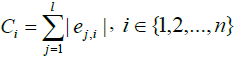
Eigenvector-based Feature Selection with Features Determined by Threshold and Sliding Window (EFS-TW): Because the contribution, importance, and relationship among features in the higher dimension will become insignificant at the lower dimension, we investigate that of original features by our methods. In our EFS-TW, the steps of performing PCA and then LDA to obtain eigenvectors till symbol ‘A’ are shown in Figure 4, and the steps of determining the contribution or the importance of original features by taking the sum of the absolute value of all eigenvector’s value till symbol ‘B’, ‘C’, and ‘D’ are shown in Figure 5 and formula 11.
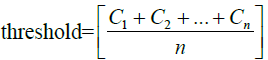
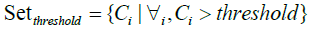
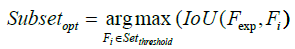
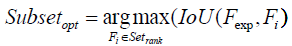
Consequently, as shown in Figure 6, the process marked in symbol ‚B‘ of Figure 5 involves the essential steps of EFSTW: removing the features which sum mentioned lower than a threshold derived from the measure such as a mean value to form a sub-optimal subset of features as shown in formulas 14 and 15, and determining a global sub-optimal subset of features shown in formula 16 with highest IoU and Coverage by a sliding window with the width 24 which is equal to the numbers of features recommended by expert.
Figure 6: Steps of removing relatively unimportant feature and determing the global sub-optimal subset of features of EFS-T.W.
The essential formulas of EFS-TW are listed as follows.
 (13)
(13)
 (14)
(14)
 (15)
(15)
 (16)
(16)
where in i is the ith featrute related to the original feature, j is the jth vector corrersponding to the PCA and LDA space, l is the number of dimension projected to the LDA space, and n is the size of feature set. The feature which value of contribution greater than the threshold will be reserved as shown in formula 15, and wherein Fexp is the feature set suggested by expert.
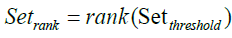
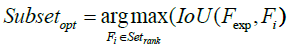
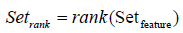
Eigenvector-based Feature Selection with Features Determined by Threshold, Ranking and Sliding Window (EFS-TRW): For brevity, the difference between EFS-TW and EFS-TRW marked in symbol ‘C’ of Figure 5 and shown in Figure 7 is that EFS-TRW ranks the remaining features in descending order (shown in formula 17) before determining a global suboptimal subset of features by a sliding window (shown in formula 18).
Figure 7: Steps of removing relatively unimportant feature, ranking and determing the global sub-optimal subset of features of EFS-TRW.
The essential formulas of EFS-TRW are listed as follows.
 (17)
(17)
 (18)
(18)
Eigenvector-based Feature Selection with Features Determined by Ranking and Sliding Window (EFS- RW): For brevity, the difference between EFS-TW and EFS-RW marked in symbol ‘D’ of Figure 5 and shown in Figure 8 is that EFS-RW omits the step of removing the features by the threshold for remaining the relative important features. Consequently, the steps of ranking features in a descending order and finding the global sub-optimal subset are shown in formulas 20 and 21.
Figure 8: Steps of ranking and determing the global sub-optimal subset of features of EFS-RW.
The essential formulas of EFS-RW are listed as follows, and wherin Ci in formula 19 is the same as described in formula 13.
 (19)
(19)
 (20)
(20)
 (21)
(21)
Model Training and Evaluation
Because of the superior performance of LSTM mentioned above, we use LSTM-related classifiers, LSTM [35], biLSTM [36], Stack-LSTM [37], Stack-biLSTM [38], and GRU, with important historical information that includes lab tests and questionnaires as inputs to predict whether the patient will be diagnosed with FLD in the specified future time or not. Considering the input sequence for LSTM is variable, we set the length to fixed 12 months. Moreover, we evaluate their performance by comparing the result of AUROC, precision, recall, F1 score, accuracy, computing time and error reduction.
Dataset used in this Study
As shown in Table 2, this study uses the FLD dataset [39] collected from a health screening center in Taipei from 2009 to 2016. Our goal is to predict whether a given person has FLD or not at specific time in the future, and this big dataset consists of 160,620 unique samples (88,056 males and 72,546 females), with 446 features (or biodata) in total (289 from questionnaires and 157 from lab tests). Besides, to show the number of patients in the eight years, we list the times of males and females examined per year that recorded in FLD dataset in Figures 9 and 10. Herein, we can see a big difference between 2013 and 2014, likely due to the implementation of Taiwan’s Personal Data Protection Act, which required medical patients have the right to opt-in to participate in medical research or not. Moreover, for males the visit count is reduced from 11,184 to 6,770 between 2013 and 2014, and the decrease rate is 60.53%. On the other hand, for females the visit count is reduced from 8,896 to 4,958, and the decrease rate is 55.73%.
Figure 9: Times for males (blue) and females (red) examined per year that recorded in FLD dataset.
Figure 10: Ratio of missing values for all features and for the top 20 features in the FLD dataset.
Also, we briefly explain the content shown in Figure 9. The bottom part is the statistical result of the top one that classified into the number of NFLD and FLD, and the classification is beneficial for calculating the respective ratio. Besides, the sizes of NFLD and FLD are 34,885 and 53,171 for males, and the ratio of NFLD/FLD is 0.66, then 48,574 and 23,990 for females, and the ratio of NFLD/FLD is 2.02. Meanwhile the ratios of NFLD/ FLD from 2009 to 2016 are {0.69, 0.67, 0.63, 0.63, 0.66, 0.68, 0.64, and 0.63} for males and {2.09, 2.16, 2.0, 1.93, 1.94, 2.1, 1.89, 1.96} for females.
Regarding the properties of our dataset, the characteristic of the dataset is its high ratio of missing values. Missing values are common in medical or healthcare datasets, and our dataset is no exception. As shown in Figure 10, it plots the ratio of missing values for all features and the top 20 features. Since features with missing value ratio 90% or higher are hard to impute, we eliminate these 17 features, leaving 252 features for further processing. In the preprocessing step, we impute missing values in our dataset using the mean for numerical features and the mode for questionnaire features. More complicated methods such as MICE (Multivariate Imputation by Chained Equations) [40] perform the imputation as well. Besides, Table 2 shows the important features in the lab test for males and females.
Also, some features, such as TG, are strong indicators of FLD that worth paying attention. To observe TG progression over eight years, we plot the yearly average TG for FLD and NFLD, broken down by males, females, and overall, respectively in Figure 11. Herein, we divide those six curves into two groups of FLD and NFLD, and TG for FLD is constantly higher than that of NFLD. Within the same group of FLD or NFLD, males usually have a higher TG than females. Moreover, those three curves belonging to group FLD have higher variance than the other three curves belonging to group NFLD, indicating that FLD patients might have a more dramatic TG progression.
Figure 11: Progression of yearly average TG over 8 years.
Again, we convert several features of the FLD dataset from different quantities due to questionnaire versions‘ inconsistencies over the past years. For instance, ‚grams of alcohol‘ represents average grams of weekly alcohol intake [41,42]. To derive this feature, we need to combine some questionnaire items related to drinking from the FLD dataset. Similarly, we combine some questionnaire items related to exercise from the FLD dataset to derive ‚weekly exercise metabolic equivalent‘.
Results and Discussions
Environment and Specification
We conduct our experiments on a 64 bits Windows 10 server, with an Intel Xeon® Silver 4116 CPU @ 2.10GHz, two NVIDIA Quadro GV100 GPU, 256GB RAM, 1TB hard disk, and Matlab R2020a (9.8.0.1417392). Besides, we construct all the models in this study based on the FLD dataset. Each of our experiments seeks to find something meaningful in the dataset, so we partition the dataset into subsets for training, validation, and test for different experiments. We perform necessary dataset preprocessing include missing value imputation and featurewise z-normalization as explained in the previous section before using it for modeling. Here we show the specification for feature selection of male for example as follows.
• Dataset: Male subjects in the FLD dataset.
• Classifier: LSTM.
• Feature selection: LSTM with 3-fold cross validation to select the most important 24 features.
• Ratio of training and test: total size of the input/output pairs for training LSTM with 24 features is 469,159. We divide the input-output pairs for prediction into 70% for the training (of which 10% is used for validation) and 30% for the test, all with stratified partitioning.
Data Preprocessing and Cleaning
As shown in Figure 12, the patient are not always visit at regular intervals, and for instance we extract four input-output pairs for prediction from the given visit patterns and discard those patients with only a single visit. When the visit pattern denoted is [v1, v2, v3, v4, v5], the extracted four input/output pairs for training LSTM are {v1 ⇒ v2}, {v1, v2 ⇒ v3}, {v1, v2, v3 ⇒ v4}, and {v1, v2, v3, v4 ⇒ v5}. For both input and output, we need to perform interpolation to create the fixed-interval data for LSTM. For instance, as shown in Figure 13, we interpolate the input to a fixed interval of one month and the output to twelve months from the nearest input.
Figure 12: A typical visit pattern and the selected input/output pairs for training LSTM.
Figure 13: The process of creating fixed-interval data for LSTM.
In this experiment, we prepare the input/output pairs used to train LSTM with 24 features in the dataset as follows. It reduces the total number of samples from 88,056 to 12,707 male and 72,564 to 10,601 female since we remove those patients with only a single visit from the dataset. We interpolate data between two consecutive visits to its monthly values from the historical data for each patient. For a specific visit, we use the past twelve months of the interpolated data as the input of LSTM and the interpolated output which twelve months after the nearest input as the output of LSTM. The input-output data pairs were collected using sliding windows with a slide of one month. Herein, we list the statistics of the average or standard length of patient sequence input for LSTM with males and females in Table 3.
| Male | Female | |
|---|---|---|
| No. of unique patients | 12,707 | 10,601 |
| No. of samples through interpolation | 152,484 | 127,212 |
| Mean of patient sequence length | 12 | 12 |
| STD of patient sequence length | 0 | 0 |
| Min. of patient sequence length | 12 | 12 |
| Max. of patient sequence length | 12 | 12 |
Table 3: Statistics of average or standard length of patient sequence input for LSTM
Feature Sets Derived and Measurement
To investigate the effectiveness of features derived by our methods, we conducted three eigenvector-based feature selections and find the global sub-optimal subset of features with the highest IoU and Coverage, and evaluate those features selected by our method and SFS with that of expert suggested features for FLD. To simplify, the features selected are partial shown in Table 4 with the brief explanation, and the matched features selected were marked with the symbol ‘*’.
| Feature Selection |
Literature | SFS | Eigenvector-based Feature Selection with the Highest IoU and Coverage | |||
|---|---|---|---|---|---|---|
| Features and Explanation | ||||||
| Features | Explanation | Suggested by experts |
Selected by SFS |
Match | Selected by EFS-TW |
Match |
| age | Age | * | * | |||
| bloodtype | Blood type | * | ||||
| bmd | Bone mineral density | * | ||||
| bmi (kg/m2) | Body mass index | * | * | * | * | * |
| cc (cm) | Chest circumference | * | ||||
| cci (cm) | Chest circumference during inspiration | * | ||||
| cea (ng/ml) | Carcinoembryonic antigen | * | ||||
| ch | The ratio of CHOL/HDLC | * | * | * | ||
| chol (mg/dl) | Total cholesterol | * | ||||
| drinkalcgram (g) | Alcohol per gram | * | ||||
| Drink year | How many years have you been drinking? | * | ||||
| ery (106/µl) | Red blood cells | * | ||||
| fat (g) | Body fat | * | * | * | * | * |
| fe (μg/dl) | Calcium Phosphorus Iron (iron) | * | ||||
| fg (mg/dl) | Diabetes mellitus fasting glucose | * | * | * | * | * |
| food18 | How many servings of bread do you eat? | * | ||||
| food19 | Do you add jam or honey to your food? | * | ||||
| food20 | Do you add sugar to your coffee, tea, drink colas, fruit juices or other beverages? | * | ||||
| food21 | How many servings of your food intake are fried in oil? | * | ||||
| ggr | The ratio of GOT/GPT | * | * | * | ||
| ggt (IU/L) | Gamma-glutamyl transferase | * | * | |||
| glo (g/dl) | Globulin | * | ||||
| got (IU/L) | Serum glutamic-oxaloacetic transaminase (sGOT) | * | ||||
| gpt (IU/L) | Serum glutamic-pyruvic transaminase (sGPT) | * | * | * | ||
| hc (cm) | Hip circumference | * | ||||
| hdlc (mg/dl) | High density lipoprotein cholesterol | * | * | * | ||
| hei (cm) | Height | * | ||||
| ldlc (mg/dl) | Low density lipoprotein cholesterol | * | * | * | ||
| leu (103/ml) | White blood cells | * | ||||
| mcv (fl) | Mean corpuscular volume | * | ||||
| mdrug10 | Steroids | * | ||||
| mdrug8 | Medicine for asthma | * | ||||
| metaequi | The metabolic equivalent for exercise per week | * | ||||
| n (%) | Neutrophils | * | ||||
| ob | Occult Blood | * | ||||
| psick17 | Have you ever suffered from the following diseases? Hepatitis | * | ||||
| psick16 | Have you ever suffered from the following diseases? Peptic ulcer | * | ||||
| psick20 | Have you ever suffered from the following diseases? Kidney stone | * | ||||
| psick21 | Have you ever suffered from the following diseases? Gout | * | ||||
| relate33b | In the last three months, have you lost weight by more than 4kg? | * | ||||
| rr (breaths/min) | Respiration Rate | * | ||||
| rsick10 | Relatives (grandparents, parents, siblings, and children) disease? Diabetes | * | ||||
| sdephi (/HPF) | Sediment epithelial cells high | * | ||||
| sdeplo (/HPF) | Sediment Epithelial Cells Low | * | ||||
| Smoke or not | Have you smoked or not? | * | ||||
| tg (mg/dl) | Triglyceride | * | * | * | * | * |
| tsh (µIU/ml) | Thyroid stimulating hormone | * | ||||
| ua (mg/dl) | Uric acid | * | ||||
| vanl | Visual acuity (naked left eye) | * | ||||
| wc (cm) | Waist circumference | * | * | * | * | * |
| wei (kg) | Weight | * | * | * | * | * |
| whr | Waist-to-hip ratio | * | * | * | ||
Table 4: Features suggested and selected for FLD prediction.
As shown in Table 5, we list the value of IoU, Coverage, number of eigenvector, and feature selected of our method, and the method with the highest value of metrics and the global suboptimal feature set is EFS-TW. Also, in Table 6, the results by performing SFS are similar to expert-suggested features. However, SFS achieves these marginal improvements at the cost of computing time. In contrast, our EFS-TW with the highest value of the IoU, the Coverage, and classification accuracy, {23.68%, 37.5%, 78.35%} for males when number of the eigenvector is 50, and {30.56%, 40.83%, 83.65%} for females when number of the eigenvector is 130, has around only 263 and 260 seconds of the whole computing time that far less than that of expert’s and SFS.
| Statistics |
Gender | IoU | Coverage | No. of Eigenvector | Feature Selected |
|---|---|---|---|---|---|
| Methods | |||||
| EFS-TW | Males | 23.68 | 37.50 | 50 | {'dm_fg', 'g_bmi', 'g_fat', 'g_wc', 'g_wei', 'g_whr', 'l_tg', 'lf_gpt', 'mdrug10'} |
| Females | 30.56 | 45.83 | 130 | {'dm_fg', 'g_bmi', 'g_fat', 'g_wc', 'g_wei', 'g_whr', 'l_ch', 'l_chol', 'l_tg', 'lf_gpt', 'mdrug10'} |
|
| EFS-TRW | Males | 23.68 | 37.50 | 90 | {'dm_fg', 'drinkalcgram', 'g_bmi', 'g_fat', 'g_wc', 'g_wei', 'g_whr', 'l_ch', 'l_tg'} |
| Females | 20.51 | 33.33 | 80 | {'drinkalcgram', 'g_bmi', 'g_fat', 'g_wc', 'g_whr', 'l_ch', 'l_tg', 'mdrug10'} | |
| EFS-RW | Males | 23.68 | 37.50 | 90 | {'dm_fg', 'drinkalcgram', 'g_bmi', 'g_fat', 'g_wc', 'g_wei', 'g_whr', 'l_ch', 'l_tg'} |
| Females | 20.51 | 33.33 | 80 | {'drinkalcgram', 'g_bmi', 'g_fat', 'g_wc', 'g_whr', 'l_ch', 'l_tg', 'mdrug10'} |
Table 5: Related metrics and features selected by our eigenvector-based feature selections
| Feature Selection |
Expert | SFS for Male | Our Methods for Male | SFS for Female | Our Methods for Female |
|---|---|---|---|---|---|
| Metric | |||||
| IoU | N/A | 23.08% | 23.68% | 9.09% | 30.56% |
| Coverage | N/A | 37.50% | 37.50% | 16.67% | 45.83% |
| Accuracy | 75.85% | 78.84% | 78.35% | 77.65% | 83.65% |
| Computing Time (Sec) | 8,675 | 380,386 | 263 | 380,350 | 260 |
Table 6: Comparison of related metrics between SFS and our method for males and females
Performance of Various Classifiers
We compare the performance of classifiers LSTM, biLSTM, GRU, Stack-LSTM, and Stack-biLSTM to two baseline models, depict the accuracy in Figure 14, and list the values of various metrics in Table 6. Here we give a brief description of Baseline 1 and Baseline 2 as follows.
Figure 14: Accuracy for two baselines and five LSTM-realed models for males and females.
• Baseline 1: This always outputs the class with a larger percentage in the ground truth. In the case of the FLD dataset, the output is always NFLD.
• Baseline 2: This is a simple inference model that always outputs the class of the previous physical examination. In other words, it determines the prediction based on the ground truth of the physical examination.
As shown in Figure 14 and Table 6, compared with the Baseline 2, classifier biLSTM achieves the top one of test accuracy 78.35% (12.63% error reduction) for males. Classifier StackbiLSTM reaches the top one of test accuracy 83.65% (37.55% error reduction) for females. Besides, their AUROC is 0.86 and 0.9, respectively.
DISCUSSION
In this section we discuss some of the experimental results and offer some findings based on our observations and the experts’ domain expertise.
Efficient feature Selections
In this study, we propose and implement various eigenvectorbased feature selection methods to our dataset which has 252 features reduced from oringinal 446 features, and either one of our feature selections significantly reduces the time for feature selection. Herein, we take the first 24 most important features by our eigenvector-based feature selection rather than SFS or other feature selection methods. According to our experimental result, it took more than 7 days for performing SFS to retrieve 24 important features. Therefore, most of the features found by our acceleration method meet expert suggestions, but the computing time is far less than that of SFS. Hence, although the number of features and width of the window can be enlarged, it is timeconsuming and inefficient to the feature selection, and helpless for the patients to follow the recommendation.
In addition, based on the results listed in Tables 4 to 6, our features selection method with the highest IoU and Coverage is EFS-TW which spent the shortest computing time in selecting features and outputting a global sub-optimal feature set. Also, our feature selections have met the requirements and targets, speedup and precision, of this study. Regarding the similarity to experts, our methods are close to or higher than SFS, but the computing time is far lower than SFS. The computing time of our method listed in Table 6 involves the time of executing three eigenvector-based feature selections in terms and then determining the best one. Besides, by observing the results listed in Table 5, IoU (30.56) and Coverage (45.83) for female of EFS-TW is different from and higher than IoU (20.51) and Coverage (33.33) for female of EFS-TRW and EFS-RW, the possible reason can be the data imbalance in our dataset and the value of threshold which needs more experiments to determine and clarify. Hence, we determine the threshold by taking the sum of absolute value of eigenvector’s value shown in Formulas 13 and 14, and herein we take absolute value of eigenvector’s value because of vector’s directionality to avoid the cancellation which cannot highlight the importance of features.
Moreover, for the features selected by our methods that listed in Table 4, we discuss the possible reasons for that why SFS and our methods unselect some features as the important risk factors such as features ‘food18’ to ‘food20’, and why SFS selects the feature ‘psick16’, ‘psick17’, ‘food20’, and ‘psick21’, but our methods choose the feature ‘rsick10’ as well. By observing our dataset, the potential reason is a high correlation between those unselected features and the selected features which is accounted for its effects already. In other words, the selected features are dataset-dependent since our dataset is large. Specifically, for food features such as ‘food18’ to ‘food20’, they are unselected for predicting FLD directly since the effects of food intake may vary among individuals. BMI, body fat, or waist circumference may also reflect food intake effects, which are more consistent features and thus selected by experts and our methods for predicting FLD. Besides, regarding the aspect of predictive medicine and data source, a health screening center rather than a hospital, the medical history with records of family or relatives having a disease such as diabetes is more concerned than the disease the patient suffered in the past or suffering now.
Furthermore, comparing the recognition rate (Accuracy shown in Table 6), and method, number and types of features to prior research, our eigenvector-based feature selections not only optimize the high-dimension features of large dataset rapidly but achieve the recognition rate better than or close to that of prior research. For example, as shown in Table 7, the best recognition rate of prior research is ranging from 70.7% to 87%, but their method, types of FLD, and numbers and types of features are all limited and more less than ours.
| Item for Comparison |
Recognition Rate | Description of Method, Number and Types of FLD and Features |
|---|---|---|
| Authors and Title | ||
| Birjandi et al., ‘Prediction and Diagnosis of Non-Alcoholic Fatty Liver Disease (NAFLD) and Identification of Its Associated Factors Using the Classification Tree Method’, 2016 | 75% | • The selection of lab test features (non-alcoholic) is determined artificially • 15 features directly related to FLD are selected based on the collected data after analysis. |
| Raika et al., ‘Prediction of Non-alcoholic Fatty Liver Disease Via a Novel Panel of Serum Adipokines’, 2016 | 86.4% | • Using only male data for model training is used • The selection of lab test feature (non-alcoholic) is determined based on the 4 features specified in the formula for calculating non-alcoholicity |
| Yip et al., ’Laboratory parameter-based machine learning model for excluding non-alcoholic fatty liver disease (NAFLD) in the general population’, 2017 | 87% | • Using only male data for model training • The selection of lab test feature (non-alcoholic) is determined based on the 6 specified features in another formula for calculating non-alcoholicity |
| Islam et al., ‘Applications of Machine Learning in Fatty Live Disease Prediction’, 2018 | 70.7% | • Using male and female data for model training • The selection of lab test features (non-alcoholic and alcoholic) is determined artificially • 8 features that are directly related to FLD are selected through analysis based on the collected data |
| Ma et al., ‘Application of Machine Learning Techniques for Clinical Predictive Modelling: A Cross-Sectional Study on Non-alcoholic Fatty Liver Disease in China’, 2018 | 83.41% | • Using male and female data for model training • The selection of lab test features (non-alcoholic) is determined artificially • 15 features directly related to FLD are selected based on the collected data after analysis |
| Wu et al., ‘Prediction of fatty liver disease using machine learning algorithms’, 2019 | 86.48% | • Using male and female data for model training • The selection of lab test features (non-alcoholic and alcoholic) is determined artificially • 10 features directly related to FLD selected after analysis based on the collected data |
Table 7: Recognition rate and brief description of prior research
High-performance prediction of FLD
For the performance of prediction, according to the result listed in Table 8, each metric shows that our prediction has achieved and satisfied the targets, such as speedup and precision, of this study. Comparison with prior research mentioned, our proposed methods have the ability to optimize the high-dimension features of large dataset rapidly and achieve better recognition rate than SFS and better performance than prior research. For this issue, we discuss and find the reason as follows.
| Metrics |
Gender | AUROC | Precision | Recall | F1 Score | Accuracy | Computing Time (hh:mm:ss) | Error Reduction |
|---|---|---|---|---|---|---|---|---|
| Classifiers | ||||||||
| LSTM | Males | 0.85 | 0.78 | 0.73 | 0.75 | 76.90% | 06:45:36 | 6.78% |
| Females | 0.90 | 0.81 | 0.79 | 0.80 | 82.68% | 08:13:20 | 33.84% | |
| biLSTM | Males | 0.86 | 0.78 | 0.76 | 0.77 | 78.35% | 03:05:08 | 12.63% |
| Females | 0.90 | 0.81 | 0.81 | 0.81 | 83.43% | 02:53:45 | 36.71% | |
| GRU | Males | 0.86 | 0.77 | 0.76 | 0.77 | 78.17% | 02:27:56 | 11.90% |
| Females | 0.90 | 0.81 | 0.81 | 0.81 | 83.38% | 02:16:22 | 36.52% | |
| Stack-LSTM | Males | 0.86 | 0.79 | 0.75 | 0.77 | 78.26% | 03:20:30 | 12.27% |
| Females | 0.90 | 0.81 | 0.81 | 0.81 | 83.62% | 03:08:10 | 37.43% | |
| Stack-biLSTM | Males | 0.87 | 0.77 | 0.78 | 0.78 | 78.23% | 04:36:19 | 12.15% |
| Females | 0.90 | 0.81 | 0.81 | 0.81 | 83.65% | 04:20:34 | 37.55% |
Table 8: Comparison of AUROC, Precision, Recall, F1 score, and Accuracy based on different classifiers
Regarding AUROC, Precision, Recall, and F1 Score, for these LSTM-related classifiers, the values of all these metrics of females are better than that of males. Particularly, AUROC is ranging from 0.85 to 0.87 for males and 0.9 for females. Classifier Stack-biLSTM achieves the top one for both males and females.
Regarding accuracy, error reduction, and computing time shown in Table 8, classifier biLSTM achieves the top one accuracy of 78.35% with an error reduction of 12.63% for males, and StackbiLSTM achieves the top one accuracy of 83.65% with an error reduction of 37.55% for females. It is reasonable that because the biLSTM and Stack-biLSTM and can gather more information than LSTM to improve its accuracy. Also, we note that the error reduction improves from 6.78% to 12.63% for males using biLSTM rather than LSTM, and 33.84% to 37.55% for females using Stack-biLSTM rather than LSTM. Still, the corresponding computing time can be shortened from around 6.75 to 3 hours for males and 8.25 to 4.3 hours for females. If we want to use the classifier with the shortest computing time, GRU saves around 4.3 hours for males and 6 hours for females, but the error reductions are acceptable. Besides, we also find that the accuracy for males is consistently lower than for females, and the possible reason could come from data imbalanced for females that are shown in Figure 11. That is, it shows that the FLD and NFLD of statistics for females have an imbalance situation between 2009 to 2016.
Conclusion
This paper explores a numerical, heterogeneous, large-scale, and high-dimension health dataset collected from a health screening center for FLD prediction. In practice, early prediction to the future status is much more valuable from the viewpoint of preventive medicine. For such a dataset, we apply our efficient eigenvector-based feature selections to optimize the feature set and automatically select the features. EFS-TW is the method with the highest IoU and Coverage but little time in computing compared to SFS. Besides, we conduct interpolation for preparing fixedinterval input data with all historical information to fulfill the operating requirement of LSTM, and compare the performance of various LSTM-related classifiers, LSTM, biLSTM, GRU, Stack-LSTM, and Stack-biLSTM, for training and evaluation. In conclusion, the proposed prediction scheme provide valuable prediction model and results for preventive medicine and lifestyle changes to eliminate the critical features that contributed to FLD progressively. Also, sufficiently high prediction accuracy allows the patient to forego a time-consuming and costly abdominal ultrasound.
Acknowledgments
This study was supported by grants from the Ministry of Science and Technology, Taiwan (MOST 110-2634-F-002-032). All data used in this research were authorized by and received from a Health Research Foundation (Authorization Code: MJHRF2019014C).
Conflict of Interest
Authors declare no conflict of interest.
REFERENCES
- Shishvan OR, Zois DS, Soyata T. Machine Intelligence in Healthcare and Medical Cyber Physical Systems: A Survey. IEEE Access. 2018; 6: 46419–46494.
- Fan JG, Kim SU, Wong VWS. New Trends on Obesity and NAFLD in Asia. J Hepatol. 2017; 67(4): 862–873.
- Hsu CS, Kao JH. Non-Alcoholic Fatty Liver Disease: An Emerging Liver Disease in Taiwan. Journal of the Formosan Medical Association. 2012; 111(10): 527–535.
- Birjandi M, Ayatollahi SMT, Pourahmad S, Safarpour AR. Prediction and Diagnosis of Non-Alcoholic Fatty Liver Disease (NAFLD) and Identification of Its Associated Factors Using the Classification Tree Method. Iranian Red Crescent Med J. 2016; 18.
- Jamali R, Arj A, Razavizade M, Aarabi MH. Prediction of Nonalcoholic Fatty Liver Disease Via A Novel Panel of Serum Adipokines. Medicine. 2016; 95(5).
- Ma H, Xu CF, Shen Z, Yu CH, Li YM. Application of Machine Learning Techniques for Clinical Predictive Modeling: A Cross-Sectional Study on Nonalcoholic Fatty Liver Disease in China. BioMed research international. Hindawi. 2018.
- Wu CC, Yeh WC, Hsu WD, Islam MM, Nguyen PAA, Poly TN. Prediction of Fatty Liver Disease Using Machine Learning Algorithms. Computer Methods and Programs in Biomedicine. 2019; 170: 23–29 .
- Yip TCF, Ma AJ, Wong VWS, Tse YK, Chan HLY, Yuen PC. Laboratory Parameter-Based Machine Learning Model for Excluding Non-Alcoholic Fatty Liver Disease (NAFLD) in the General Population. Alimentary pharmacology and therapeutics. 2017; 46(4): 447–456 .
- Gu S, Cheng R, Jin Y. Feature Selection for High-Dimensional Classification Using A Competitive Swarm Optimizer. Soft Computing. 2018; 22(3): 811–822.
- Juha R. Overfitting in Making Comparisons Between Variable Selection Methods. Journal of Machine Learning Research. 2003; 3(Mar): 1371–1382.
- Islam MM, Wu CC, Poly TN, Yang HC, Li YCJ. Applications of Machine Learning in Fatty Live Disease Prediction. Machine learning. 2018; 166–170.
- Paul D, Su R, Romain M, Sébastien V, Pierre V, Isabelle G. Feature Selection for Outcome Prediction in Oesophageal Cancer Using Genetic Algorithm and Random Forest Classifier. Computerized Medical Imaging and Graphics. 2017; 60: 42–49.
- Tian Y, Zhang X, Wang C, Jin Y. An Evolutionary Algorithm for Large-Scale Sparse MultiObjective Optimization Problems. IEEE Transactions on Evolutionary Computation. 2019.
- Wei X, Jiang F, Wei F, Zhang J, Liao W, Cheng S. An Ensemble Model for Diabetes Diagnosis in Large-Scale and Imbalanced Dataset. Proceedings of the computing frontiers conference. 2017; 71–78.
- Martinez AM, Kak AC. PCA versus LDA. IEEE transactions on pattern analysis and machine intelligence. 2001; 23(2): 228-233.
- Borade SN, Adgaonkar RP. Comparative analysis of PCA and LDA. International Conference on Business, Engineering and Industrial Applications. 2011; 203-206.
- Yang WY, Zhang H, Li MX, Lai FN. Research on Improved PCA Face Recognition Algorithm. DEStech Transactions on Engineering and Technology Research. 2019.
- Marcialis GL, Roli F. Fusion of LDA and PCA for Face Verification. International Workshop on Biometric Authentication. 2002; 30-37.
- Ferizal R, Wibirama S, Setiawan NA. Gender recognition using PCA and LDA with improve preprocessing and classification technique. 7th International annual engineering seminar (InAES). 2017; 1-6.
- Varma S, Shinde M, Chavan SS. Analysis of PCA and LDA Features for Facial Expression Recognition Using SVM and HMM Classifiers. Techno-Societal. 2020; 109-119.
- Zhang D, Xiong A, Zhao X, Han J. PCA and LDA for EMG-based control of bionic mechanical hand. IEEE International Conference on Information and Automation. 2012; 960-965.
- Li R, Zhao Y, Zhang X, Cao Y, Chen X. Banknote Infrared Characteristics Discrimination Based on PCA and LDA. International Conference on Artificial Intelligence and Security. 2020; 493-502.
- Davagdorj K, Yu SH, Kim SYM, Huy PV, Park JH, Ryu KH. Prediction of 6 Months Smoking Cessation Program among Women in Korea. International Journal of Machine Learning and Computing. 2019; 9: 83–90.
- Emrah H. Differential Evolution for Feature Selection: A Fuzzy Wrapper–Filter Approach. Soft Computing. 2019; 23(13): 5233–5248.
- Park HW, Batbaatar E, Li D, Ryu KH. Risk Factors Rule Mining in Hypertension: Korean National Health and Nutrient Examinations Survey 2007–2014. Journal of the Formosan Medical Association. IEEE Conference on Computational Intelligence in Bioinformatics and Computational Biology (CIBCB). 2016; 1–4.
- Park KH, Ishag MIM, Ryu KS, Li M, Ryu KH. Efficient Ensemble Methods for Classification on Clear Cell Renal Cell Carcinoma Clinical Dataset. Asian Conference on Intelligent Information and Database Systems. 2018; 235–242.
- Whitney AW. A Direct Method of Nonparametric Measurement Selection. IEEE Transactions on Computers. 1971; 100(9); 1100–1103.
- Liu, JH, Wu, CT, Chu, TW, Jang, JS. Data-driven Feature Selection for Long Longitudinal Breadth and High Dimensional Dataset: Empirical Studies of Metabolic Syndrome Prediction. International Conference on Machine Learning and Computing (ICMLC). 2020; 208-212.
- Kim MH, Kim JH, Lee K, Gim GY. The Prediction of COVID-19 Using LSTM Algorithms. International Journal of Networked and Distributed Computing. 2021.
- Pal R, Sekh AA, Kar S, Prasad DK. Neural network based country wise risk prediction of COVID-19. Journal of Applied Sciences. 2020; 10(18): 6448.
- Zhang N, Shen SL, Zhou A, Jin YF. Application of LSTM approach for modeling stress–strain behavior of soil. Journal of Applied Soft Computing. 2021; 100: 106959.
- Sunny MAI, Maswood MMS, Alharbi AG. Deep Learning-Based Stock Price Prediction Using LSTM and Bi-Directional LSTM Model. Novel Intelligent and Leading Emerging Sciences Conference (NILES). 2020; 87-92.
- Wang G, Li Z, Li G, Dai G, Xiao Q, Bai L, Bai S. Real-time liver tracking algorithm based on LSTM and SVR networks for use in surface-guided radiation therapy. Journal of Radiation Oncology. 2021; 16(1): 1-12.
- Qiao D, Li P, Ma G, Qi X, Yan J, Ning D, Li B. Realtime prediction of dynamic mooring lines responses with LSTM neural network model. Journal of Ocean Engineering. 2021; 219: 108368.
- Hochreiter S, Schmidhuber J. Long Short-Term Memory. Neural Computation. 1997; 9(8): 1735–1780.
- Graves A, Schmidhuber J. Bidirectional Recurrent Neural Networks. IEEE Transactions on Signal Processing. 1997. 45: 2673-2681.
- Dyer C, Ballesteros M, Ling W, Matthews A, Noah A. Transition-based dependency parsing with stack long short-term memory. Proceedings of ACL. 2015.
- Cai L, Zhou S, Yan Y, Yuan R. A stacked BiLSTM neural network based on coattention mechanism for question answering. Journal of computational intelligence and neuroscience. 2019.
- MJHRF, The Code Book for Biodata and Health Survey Data of MJ Health Research Foundation. [Cited 2020 Jan 1]; Available from; http://www.mjhrf.org/main/page/resource/en/#resource03
- Buuren SV, Groothuis-Oudshoorn K. MICE: Multivariate Imputation by Chained Equations in R. Journal of statistical software. 2010; 1–68 .
- Ainsworth BE. The Compendium of Physical Activities Tracking Guide. University of South Carolina. 2002.
- Ainsworth BE, Haskell WL, Herrmann SD, Meckes N, Bassett DRJ, TL CATRINE. 2011 Compendium of Physical Activities: A Second Update of Codes and MET Values. Medicine and Science in Sports and Exercise. 2011; 43(8): 1575–1581.